We have seen how to solve a restricted collection of differential equations, or more accurately, how to attempt to solve them—we may not be able to find the required anti-derivatives. Not surprisingly, non-linear equations can be even more difficult to solve. Yet much is known about solutions to some more general equations.

Suppose $\phi(t,y)$ is a function of two variables. A more general class of first order differential equations has the form $\ds\dot y=\phi(t,y)$. This is not necessarily a linear first order equation, since $\phi$ may depend on $y$ in some complicated way; note however that $\ds\dot y$ appears in a very simple form. Under suitable conditions on the function $\phi$, it can be shown that every such differential equation has a solution, and moreover that for each initial condition the associated initial value problem has exactly one solution. In practical applications this is obviously a very desirable property.

Not all differential equations that are important in practice can be solved exactly, so techniques have been developed to approximate solutions. We describe one such technique, Euler's Method, which is simple though not particularly useful compared to some more sophisticated techniques.

Suppose we wish to approximate a solution to the initial value problem $\ds\dot y=\phi(t,y)$, $\ds y(t_0)=y_0$, for $t\ge t_0$. Under reasonable conditions on $\phi$, we know the solution exists, represented by a curve in the $t$-$y$ plane; call this solution $f(t)$. The point $\ds (t_0,y_0)$ is of course on this curve. We also know the slope of the curve at this point, namely $\ds\phi(t_0,y_0)$. If we follow the tangent line for a brief distance, we arrive at a point that should be almost on the graph of $f(t)$, namely $\ds(t_0+\Delta t, y_0+\phi(t_0,y_0)\Delta t)$; call this point $\ds(t_1,y_1)$. Now we pretend, in effect, that this point really is on the graph of $f(t)$, in which case we again know the slope of the curve through $\ds(t_1,y_1)$, namely $\ds\phi(t_1,y_1)$. So we can compute a new point, $\ds(t_2,y_2)=(t_1+\Delta t, y_1+\phi(t_1,y_1)\Delta t)$ that is a little farther along, still close to the graph of $f(t)$ but probably not quite so close as $\ds(t_1,y_1)$. We can continue in this way, doing a sequence of straightforward calculations, until we have an approximation $\ds(t_n,y_n)$ for whatever time $\ds t_n$ we need. At each step we do essentially the same calculation, namely $$(t_{i+1},y_{i+1})=(t_i+\Delta t, y_i+\phi(t_i,y_i)\Delta t).$$ We expect that smaller time steps $\Delta t$ will give better approximations, but of course it will require more work to compute to a specified time. It is possible to compute a guaranteed upper bound on how far off the approximation might be, that is, how far $\ds y_n$ is from $f(t_n)$. Suffice it to say that the bound is not particularly good and that there are other more complicated approximation techniques that do better.

Example 19.4.3 Let us compute an approximation to the solution for $\ds\dot y=t-y^2$, $y(0)=0$, when $t=1$. We will use $\Delta t=0.2$, which is easy to do even by hand, though we should not expect the resulting approximation to be very good. We get $$\eqalign{ (t_1,y_1)&=(0+0.2,0+(0-0^2)0.2) = (0.2,0)\cr (t_2,y_2)&=(0.2+0.2,0+(0.2-0^2)0.2) = (0.4,0.04)\cr (t_3,y_3)&=(0.6,0.04+(0.4-0.04^2)0.2) = (0.6,0.11968)\cr (t_4,y_4)&=(0.8,0.11968+(0.6-0.11968^2)0.2) = (0.8,0.23681533952)\cr (t_5,y_5)&=(1.0,0.23681533952+(0.6-0.23681533952^2)0.2) = (1.0,0.385599038513605)\cr} $$ So $y(1)\approx 0.3856$. As it turns out, this is not accurate to even one decimal place. Figure 19.4.1 shows these points connected by line segments (the lower curve) compared to a solution obtained by a much better approximation technique. Note that the shape is approximately correct even though the end points are quite far apart.

Figure 19.4.1. Approximating a solution to $\ds\dot y=t-y^2$, $y(0)=0$.

If you need to do Euler's method by hand, it is useful to construct a table to keep track of the work, as shown in figure 19.4.2. Each row holds the computation for a single step: the starting point $(t_i,y_i)$; the stepsize $\Delta t$; the computed slope $\phi(t_i,y_i)$; the change in $y$, $\Delta y=\phi(t_i,y_i)\Delta t$; and the new point, $(t_{i+1},y_{i+1})=(t_i+\Delta t,y_i+\Delta y)$. The starting point in each row is the newly computed point from the end of the previous row.

$(t,y)$	$\Delta t$	$\phi(t,y)$	$\Delta y=\phi(t,y)\Delta t$	$(t+\Delta t,y+\Delta y)$
$(0,0)$	$0.2$	$0$	$0$	$(0.2,0)$
$(0.2,0)$	$0.2$	$0.2$	$0.04$	$(0.4,0.04)$
$(0.4,0.04)$	$0.2$	$0.3984$	$0.07968$	$(0.6,0.11968)$
$(0.6,0.11968)$	$0.2$	$0.58\ldots$	$0.117\ldots$	$(0.8,0.2368\ldots)$
$(0.8,0.236\ldots)$	$0.2$	$0.743\ldots$	$0.148\ldots$	$(1.0,0.385\ldots$

Figure 19.4.2. Computing with Euler's Method.

It is easy to write a short function in Sage to do Euler's method. The euler function defined below computes and displays approximations to points on the solution curve for the differential equation $y'=f(t,y)$ with initial condition (init_t, init_y). The step size is (final_t-init_t)/m. The function displays the points calculated and also returns a list of the points. You may change the function and the other parameters in the last two lines to try other examples.

$\square$

Euler's method is related to another technique that can help in understanding a differential equation in a qualitative way. Euler's method is based on the ability to compute the slope of a solution curve at any point in the plane, simply by computing $\phi(t,y)$. If we compute $\phi(t,y)$ at many points, say in a grid, and plot a small line segment with that slope at the point, we can get an idea of how solution curves must look. Such a plot is called a slope field.

Sage can plot slope fields. Here we display the approximation computed above together with the slope field. With a little practice, one can sketch reasonably accurate solution curves based on the slope field, in essence doing Euler's method visually. (You must evaluate the Sage cell above before you evaluate this one.)

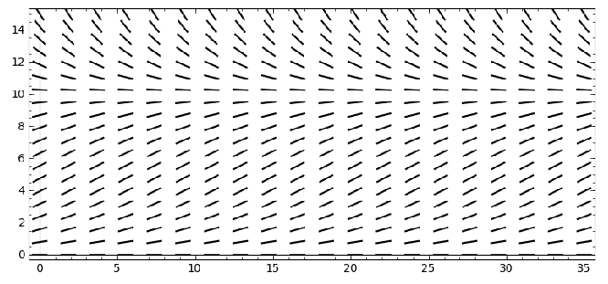
Even when a differential equation can be solved explicitly, the slope field can help in understanding what the solutions look like with various initial conditions. Recall the logistic equation from exercise 13 in section 19.1, $\ds\dot y = ky(M-y)$: $y$ is a population at time $t$, $M$ is a measure of how large a population the environment can support, and $k$ measures the reproduction rate of the population. Figure 19.4.3 shows a slope field for this equation that is quite informative. It is apparent that if the initial population is smaller than $M$ it rises to $M$ over the long term, while if the initial population is greater than $M$ it decreases to $M$.

Figure 19.4.3. A slope field for $\ds\dot y=0.2y(10-y)$.

Exercises 19.4

In problems 1–4, compute the Euler approximations for the initial value problem for $0\le t\le 1$ and $\Delta t=0.2$. Using Sage, generate the slope field first and attempt to sketch the solution curve. Then use Sage to compute better approximations with smaller values of $\Delta t$.

Ex 19.4.1 $\ds\dot y=t/y$, $y(0)=1$ (answer)

Ex 19.4.2 $\ds\dot y=t+y^3$, $y(0)=1$ (answer)

Ex 19.4.3 $\ds\dot y=\cos(t+y)$, $y(0)=1$ (answer)

Ex 19.4.4 $\ds\dot y=t\ln y$, $y(0)=2$ (answer)