
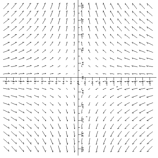
This chapter is concerned with applying calculus in the context of vector fields. A two-dimensional vector field is a function $f$ that maps each point $(x,y)$ in $\R^2$ to a two-dimensional vector $\langle u,v\rangle$, and similarly a three-dimensional vector field maps $(x,y,z)$ to $\langle u,v,w\rangle$. Since a vector has no position, we typically indicate a vector field in graphical form by placing the vector $f(x,y)$ with its tail at $(x,y)$. Figure 18.1.1 shows a representation of the vector field $f(x,y)=\langle -x/\sqrt{x^2+y^2+4},y/\sqrt{x^2+y^2+4}\rangle$. For such a graph to be readable, the vectors must be fairly short, which is accomplished by using a different scale for the vectors than for the axes. Such graphs are thus useful for understanding the sizes of the vectors relative to each other but not their absolute size.
Vector fields have many important applications, as they can be used to represent many physical quantities: the vector at a point may represent the strength of some force (gravity, electricity, magnetism) or a velocity (wind speed or the velocity of some other fluid).
We have already seen a particularly important kind of vector field—the gradient. Given a function $f(x,y)$, recall that the gradient is $\langle f_x(x,y),f_y(x,y)\rangle$, a vector that depends on (is a function of) $x$ and $y$. We usually picture the gradient vector with its tail at $(x,y)$, pointing in the direction of maximum increase. Vector fields that are gradients have some particularly nice properties, as we will see. An important example is $${\bf F}= \left \langle {-x\over (x^2+y^2+z^2)^{3/2}},{-y\over (x^2+y^2+z^2)^{3/2}},{-z\over (x^2+y^2+z^2)^{3/2}}\right\rangle,$$ which points from the point $(x,y,z)$ toward the origin and has length $${\sqrt{x^2+y^2+z^2}\over(x^2+y^2+z^2)^{3/2}}= {1\over(\sqrt{x^2+y^2+z^2})^2},$$ which is the reciprocal of the square of the distance from $(x,y,z)$ to the origin—in other words, ${\bf F}$ is an "inverse square law''. The vector $\bf F$ is a gradient: $$\eqalignno{ {\bf F} &= \nabla {1\over\sqrt{x^2+y^2+z^2} },& (18.1.1) }$$ which turns out to be extremely useful.
Exercises 18.1
Sketch the vector fields; check your work with Sage's
plot_vector_field
function. Here is an example:
Ex 18.1.1 $\langle x,y\rangle$
Ex 18.1.2 $\langle -x, -y\rangle$
Ex 18.1.3 $\langle x,-y\rangle$
Ex 18.1.4 $\langle \sin x,\cos y\rangle$
Ex 18.1.5 $\langle y,1/x\rangle$
Ex 18.1.6 $\langle x+1,x+3\rangle$
Ex 18.1.7 Verify equation 18.1.1.