
When we first considered what the derivative of a vector function might mean, there was really not much difficulty in understanding either how such a thing might be computed or what it might measure. In the case of functions of two variables, things are a bit harder to understand. If we think of a function of two variables in terms of its graph, a surface, there is a more-or-less obvious derivative-like question we might ask, namely, how "steep'' is the surface. But it's not clear that this has a simple answer, nor how we might proceed. We will start with what seem to be very small steps toward the goal; surprisingly, it turns out that these simple ideas hold the keys to a more general understanding.
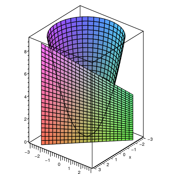
Imagine a particular point on a surface; what might we be able to say about how steep it is? We can limit the question to make it more familiar: how steep is the surface in a particular direction? What does this even mean? Here's one way to think of it: Suppose we're interested in the point $(a,b,c)$. Pick a straight line in the $x$-$y$ plane through the point $(a,b,0)$, then extend the line vertically into a plane. Look at the intersection of the plane with the surface. If we pay attention to just the plane, we see the chosen straight line where the $x$-axis would normally be, and the intersection with the surface shows up as a curve in the plane. Figure 16.3.1 shows the parabolic surface from figure 16.1.2, exposing its cross-section above the line $x+y=1$.
In principle, this is a problem we know how to solve: find the slope of a curve in a plane. Let's start by looking at some particularly easy lines: those parallel to the $x$ or $y$ axis. Suppose we are interested in the cross-section of $f(x,y)$ above the line $y=b$. If we substitute $b$ for $y$ in $f(x,y)$, we get a function in one variable, describing the height of the cross-section as a function of $x$. Because $y=b$ is parallel to the $x$-axis, if we view it from a vantage point on the negative $y$-axis, we will see what appears to be simply an ordinary curve in the $x$-$z$ plane.
|
|
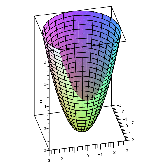
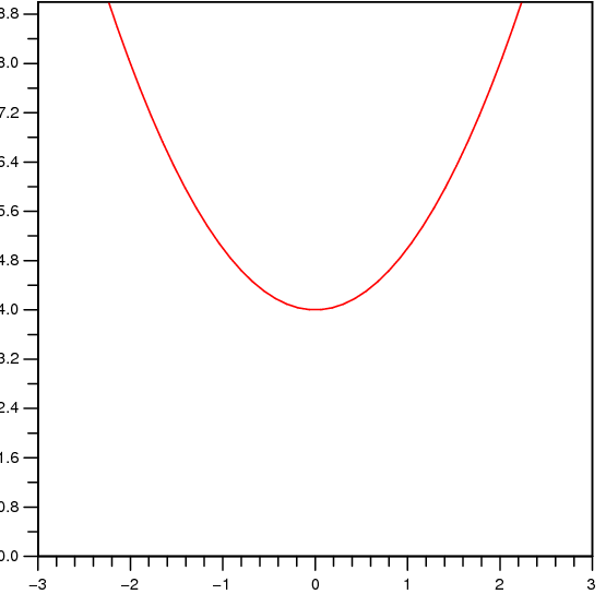
Consider again the parabolic surface $f(x,y)=x^2+y^2$. The cross-section above the line $y=2$ consists of all points $(x,2,x^2+4)$. Looking at this cross-section from somewhere on the negative $y$ axis, we see what appears to be just the curve $f(x)=x^2+4$. At any point on the cross-section, $(a,2,a^2+4)$, the steepness of the surface in the direction of the line $y=2$ is simply the slope of the curve $f(x)=x^2+4$ at $x=a$, namely $2a$. Figure 16.3.2 shows the same parabolic surface as before, but now cut by the plane $y=2$. The left graph shows the cut-off surface, the right shows just the cross-section, looking up from the negative $y$-axis toward the origin.
If, say, we're interested in the point $(-1,2,5)$ on the surface, then the slope in the direction of the line $y=2$ is $2x=2(-1)=-2$. This means that starting at $(-1,2,5)$ and moving on the surface, above the line $y=2$, in the direction of increasing $x$ values, the surface goes down; of course moving in the opposite direction, toward decreasing $x$ values, the surface will rise.
If we're interested in some other line $y=k$, there is really no change in the computation. The equation of the cross-section above $y=k$ is $x^2+k^2$ with derivative $2x$. We can save ourselves the effort, small as it is, of substituting $k$ for $y$: all we are in effect doing is temporarily assuming that $y$ is some constant. With this assumption, the derivative ${d\over dx}(x^2+y^2)=2x$. To emphasize that we are only temporarily assuming $y$ is constant, we use a slightly different notation: ${\partial\over \partial x}(x^2+y^2)=2x$; the "$\partial$'' reminds us that there are more variables than $x$, but that only $x$ is being treated as a variable. We read the equation as "the partial derivative of $(x^2+y^2)$ with respect to $x$ is $2x$.'' A convenient alternate notation for the partial derivative of $f(x,y)$ with respect to $x$ is $f_x(x,y)$.
Example 16.3.1 The partial derivative with respect to $x$ of $x^3+3xy$ is $3x^2+3y$. Note that the partial derivative includes the variable $y$, unlike the example $x^2+y^2$. It is somewhat unusual for the partial derivative to depend on a single variable; this example is more typical. $\square$
Of course, we can do the same sort of calculation for lines parallel to the $y$-axis. We temporarily hold $x$ constant, which gives us the equation of the cross-section above a line $x=k$. We can then compute the derivative with respect to $y$; this will measure the steepness of the curve in the $y$ direction.
Example 16.3.2 The partial derivative with respect to $y$ of $f(x,y)=\sin(xy)+3xy$ is $$f_y(x,y)={\partial\over\partial y}\sin(xy)+3xy=\cos(xy){\partial\over\partial y}(xy)+ 3x=x\cos(xy)+3x. $$
$\square$
So far, using no new techniques, we have succeeded in measuring the slope of a surface in two quite special directions. For functions of one variable, the derivative is closely linked to the notion of tangent line. For surfaces, the analogous idea is the tangent plane—a plane that just touches a surface at a point, and has the same "steepness'' as the surface in all directions. Even though we haven't yet figured out how to compute the slope in all directions, we have enough information to find tangent planes. Suppose we want the plane tangent to a surface at a particular point $(a,b,c)$. If we compute the two partial derivatives of the function for that point, we get enough information to determine two lines tangent to the surface, both through $(a,b,c)$ and both tangent to the surface in their respective directions. These two lines determine a plane, that is, there is exactly one plane containing the two lines: the tangent plane. Figure 16.3.3 shows (part of) two tangent lines at a point, and the tangent plane containing them.
|
|
How can we discover an equation for this tangent plane? We know a point on the plane, $(a,b,c)$; we need a vector normal to the plane. If we can find two vectors, one parallel to each of the tangent lines we know how to find, then the cross product of these vectors will give the desired normal vector.
How can we find vectors parallel to the tangent lines? Consider first the line tangent to the surface above the line $y=b$. A vector $\langle u,v,w\rangle$ parallel to this tangent line must have $y$ component $v=0$, and we may as well take the $x$ component to be $u=1$. The ratio of the $z$ component to the $x$ component is the slope of the tangent line, precisely what we know how to compute. The slope of the tangent line is $f_x(a,b)$, so $$ f_x(a,b)={w\over u} ={w\over1} = w.$$ In other words, a vector parallel to this tangent line is $\langle 1,0,f_x(a,b)\rangle$, as shown in figure 16.3.4. If we repeat the reasoning for the tangent line above $x=a$, we get the vector $\langle 0,1,f_y(a,b)\rangle$.
Now to find the desired normal vector we compute the cross product, $\langle 0,1,f_y\rangle\times\langle 1,0,f_x\rangle= \langle f_x,f_y,-1\rangle$. From our earlier discussion of planes, we can write down the equation we seek: $f_x(a,b)x+f_y(a,b)y-z=k$, and $k$ as usual can be computed by substituting a known point: $f_x(a,b)(a)+f_y(a,b)(b)-c=k$. There are various more-or-less nice ways to write the result: $$\displaylines{ f_x(a,b)x+f_y(a,b)y-z=f_x(a,b)a+f_y(a,b)b-c\cr f_x(a,b)x+f_y(a,b)y-f_x(a,b)a-f_y(a,b)b+c=z\cr f_x(a,b)(x-a)+f_y(a,b)(y-b)+c=z\cr f_x(a,b)(x-a)+f_y(a,b)(y-b)+f(a,b)=z\cr }$$
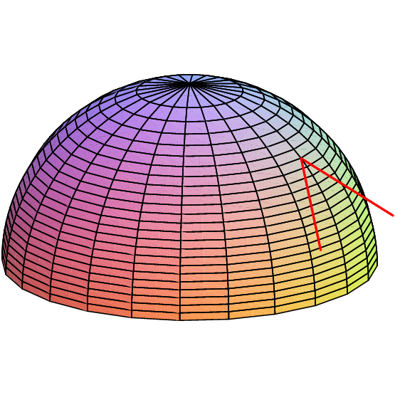
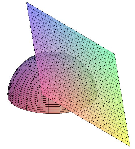
Example 16.3.3 Find the plane tangent to $x^2+y^2+z^2=4$ at $(1,1,\sqrt2)$. This point is on the upper hemisphere, so we use $\ds f(x,y)=\sqrt{4-x^2-y^2}$. Then $\ds f_x(x,y)=-x(4-x^2-y^2)^{-1/2}$ and $\ds f_y(x,y)=-y(4-x^2-y^2)^{-1/2}$, so $f_x(1,1)=f_y(1,1)=-1/\sqrt2$ and the equation of the plane is $$z=-{1\over\sqrt2}(x-1)-{1\over\sqrt2}(y-1)+\sqrt2.$$ The hemisphere and this tangent plane are pictured in figure 16.3.3. $\square$
So it appears that to find a tangent plane, we need only find two quite simple ordinary derivatives, namely $f_x$ and $f_y$. This is true if the tangent plane exists. It is, unfortunately, not always the case that if $f_x$ and $f_y$ exist there is a tangent plane. Consider the function $xy^2/(x^2+y^4)$ pictured in figure 16.2.1. This function has value 0 when $x=0$ or $y=0$, and we can "plug the hole'' by agreeing that $f(0,0)=0$. Now it's clear that $f_x(0,0)=f_y(0,0)=0$, because in the $x$ and $y$ directions the surface is simply a horizontal line. But it's also clear from the picture that this surface does not have anything that deserves to be called a "tangent plane'' at the origin, certainly not the $x$-$y$ plane containing these two tangent lines.
When does a surface have a tangent plane at a particular point? What we really want from a tangent plane, as from a tangent line, is that the plane be a "good'' approximation of the surface near the point. Here is how we can make this precise:
Definition 16.3.4 Let $\Delta x=x-x_0$, $\Delta y=y-y_0$, and $\Delta z=z-z_0$ where $z_0=f(x_0,y_0)$. The function $z=f(x,y)$ is differentiable at $(x_0,y_0)$ if $$\Delta z=f_x(x_0,y_0)\Delta x+f_y(x_0,y_0)\Delta y+\epsilon_1\Delta x + \epsilon_2\Delta y,$$ and both $\epsilon_1$ and $\epsilon_2$ approach 0 as $(x,y)$ approaches $(x_0,y_0)$. $\square$
This definition takes a bit of absorbing. Let's rewrite the central equation a bit: $$\eqalignno{ z&=f_x(x_0,y_0)(x-x_0)+f_y(x_0,y_0)(y-y_0)+f(x_0,y_0)+ \epsilon_1\Delta x + \epsilon_2\Delta y.& (16.3.1)\cr }$$ The first three terms on the right give the value of $z$ on the tangent plane, that is, $$f_x(x_0,y_0)(x-x_0)+f_y(x_0,y_0)(y-y_0)+f(x_0,y_0)$$ is the $z$-value of the point on the plane above $(x,y)$. Equation 16.3.1 says that the $z$-value of a point on the surface is equal to the $z$-value of a point on the plane plus a "little bit,'' namely $\epsilon_1\Delta x + \epsilon_2\Delta y$. As $(x,y)$ approaches $(x_0,y_0)$, both $\Delta x$ and $\Delta y$ approach 0, so this little bit $\epsilon_1\Delta x + \epsilon_2\Delta y$ also approaches 0, and the $z$-values on the surface and the plane get close to each other. But that by itself is not very interesting: since the surface and the plane both contain the point $(x_0,y_0,z_0)$, the $z$ values will approach $z_0$ and hence get close to each other whether the tangent plane is "tangent'' to the surface or not. The extra condition in the definition says that as $(x,y)$ approaches $(x_0,y_0)$, the $\epsilon$ values approach 0—this means that $\epsilon_1\Delta x + \epsilon_2\Delta y$ approaches 0 much, much faster, because $\epsilon_1\Delta x$ is much smaller than either $\epsilon_1$ or $\Delta x$. It is this extra condition that makes the plane a tangent plane.
We can see that the extra condition on $\epsilon_1$ and $\epsilon_2$ fits neatly with the definition of partial derivatives. Suppose we temporarily fix $y=y_0$, so $\Delta y=0$. Then the equation from the definition becomes $$\Delta z=f_x(x_0,y_0)\Delta x+\epsilon_1\Delta x$$ or $${\Delta z\over\Delta x}=f_x(x_0,y_0)+\epsilon_1.$$ Now taking the limit of the two sides as $\Delta x$ approaches 0, the left side turns into the partial derivative of $z$ with respect to $x$ at $(x_0,y_0)$, or in other words $f_x(x_0,y_0)$, and the right side does the same, because as $(x,y)$ approaches $(x_0,y_0)$, $\epsilon_1$ approaches 0. Essentially the same calculation works for $f_y$.
Almost all of the functions we will encounter are differentiable at points we will be interested in, and often at all points. This is usually because the functions satisfy the hypotheses of this theorem.
Theorem 16.3.5 If $f(x,y)$ and its partial derivatives are continuous at a point $(x_0,y_0)$, then $f$ is differentiable there. $\qed$
Exercises 16.3
Partial derivatives are just like ordinary derivatives in Sage.
Ex 16.3.1 Find $f_x$ and $f_y$ where $\ds f(x,y)=\cos(x^2y)+y^3$. (answer)
Ex 16.3.2 Find $f_x$ and $f_y$ where $\ds f(x,y)={xy\over x^2+y}$. (answer)
Ex 16.3.3 Find $f_x$ and $f_y$ where $\ds f(x,y)=e^{x^2+y^2}$. (answer)
Ex 16.3.4 Find $f_x$ and $f_y$ where $\ds f(x,y)=xy\ln(xy)$. (answer)
Ex 16.3.5 Find $f_x$ and $f_y$ where $\ds f(x,y)=\sqrt{1-x^2-y^2}$. (answer)
Ex 16.3.6 Find $f_x$ and $f_y$ where $\ds f(x,y)=x\tan(y)$. (answer)
Ex 16.3.7 Find $f_x$ and $f_y$ where $\ds f(x,y)={1\over xy}$. (answer)
Ex 16.3.8 Find an equation for the plane tangent to $\ds 2x^2+3y^2-z^2=4$ at $(1,1,-1)$. (answer)
Ex 16.3.9 Find an equation for the plane tangent to $\ds f(x,y)=\sin(xy)$ at $(\pi,1/2,1)$. (answer)
Ex 16.3.10 Find an equation for the plane tangent to $\ds f(x,y)=x^2+y^3$ at $(3,1,10)$. (answer)
Ex 16.3.11 Find an equation for the plane tangent to $\ds f(x,y)=x\ln(xy)$ at $(2,1/2,0)$. (answer)
Ex 16.3.12 Find an equation for the line normal to $\ds x^2+4y^2=2z$ at $(2,1,4)$. (answer)
Ex 16.3.13 Explain in your own words why, when taking a partial derivative of a function of multiple variables, we can treat the variables not being differentiated as constants.
Ex 16.3.14 Consider a differentiable function, $f(x,y)$. Give physical interpretations of the meanings of $f_x(a,b)$ and $f_y(a,b)$ as they relate to the graph of $f$.
Ex 16.3.15 In much the same way that we used the tangent line to approximate the value of a function from single variable calculus, we can use the tangent plane to approximate a function from multivariable calculus. Consider the tangent plane found in Exercise 11. Use this plane to approximate $f(1.98, 0.4)$. (answer)
Ex 16.3.16 Suppose that one of your colleagues has calculated the partial derivatives of a given function, and reported to you that $f_x(x,y)=2x+3y$ and that $f_y(x,y)=4x+6y$. Do you believe them? Why or why not? If not, what answer might you have accepted for $f_y$?
Ex 16.3.17 Suppose $f(t)$ and $g(t)$ are single variable differentiable functions. Find $\partial z/\partial x$ and $\partial z/\partial y$ for each of the following functions of two variables.
a. $z=f(x)g(y)$
b. $z=f(xy)$
c. $z=f(x/y)$
(answer)