
Consider a surface $f(x,y)$; you might temporarily think of this as representing physical topography—a hilly landscape, perhaps. What is the average height of the surface (or average altitude of the landscape) over some region?
As with most such problems, we start by thinking about how we might approximate the answer. Suppose the region is a rectangle, $[a,b]\times[c,d]$. We can divide the rectangle into a grid, $m$ subdivisions in one direction and $n$ in the other, as indicated in figure 17.1.1. We pick $x$ values $x_0$, $x_1$,…, $x_{m-1}$ in each subdivision in the $x$ direction, and similarly in the $y$ direction. At each of the points $(x_i,y_j)$ in one of the smaller rectangles in the grid, we compute the height of the surface: $f(x_i,y_j)$. Now the average of these heights should be (depending on the fineness of the grid) close to the average height of the surface: $${f(x_0,y_0)+f(x_1,y_0)+\cdots+f(x_0,y_1)+f(x_1,y_1)+\cdots+ f(x_{m-1},y_{n-1})\over mn}.$$
As both $m$ and $n$ go to infinity, we expect this approximation to converge to a fixed value, the actual average height of the surface. For reasonably nice functions this does indeed happen.
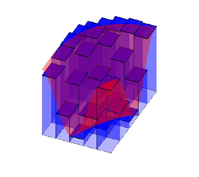
Using sigma notation, we can rewrite the approximation: $$\eqalign{ {1\over mn}\sum_{i=0}^{n-1}\sum_{j=0}^{m-1}f(x_j,y_i) &={1\over(b-a)(d-c)}\sum_{i=0}^{n-1}\sum_{j=0}^{m-1}f(x_j,y_i) {b-a\over m}{d-c\over n}\cr &= {1\over(b-a)(d-c)}\sum_{i=0}^{n-1}\sum_{j=0}^{m-1}f(x_j,y_i)\Delta x\Delta y.\cr }$$ The two parts of this product have useful meaning: $(b-a)(d-c)$ is of course the area of the rectangle, and the double sum adds up $mn$ terms of the form $f(x_j,y_i)\Delta x\Delta y$, which is the height of the surface at a point times the area of one of the small rectangles into which we have divided the large rectangle. In short, each term $f(x_j,y_i)\Delta x\Delta y$ is the volume of a tall, thin, rectangular box, and is approximately the volume under the surface and above one of the small rectangles; see figure 17.1.2. When we add all of these up, we get an approximation to the volume under the surface and above the rectangle $R=[a,b]\times[c,d]$. When we take the limit as $m$ and $n$ go to infinity, the double sum becomes the actual volume under the surface, which we divide by $(b-a)(d-c)$ to get the average height.
Double sums like this come up in many applications, so in a way it is the most important part of this example; dividing by $(b-a)(d-c)$ is a simple extra step that allows the computation of an average. As we did in the single variable case, we introduce a special notation for the limit of such a double sum: $$\lim_{m,n\to\infty} \sum_{i=0}^{n-1}\sum_{j=0}^{m-1}f(x_j,y_i)\Delta x\Delta y=\dint{R} f(x,y)\,dx\,dy=\dint{R} f(x,y)\,dA,$$ the double integral of $f$ over the region $R$. The notation $dA$ indicates a small bit of area, without specifying any particular order for the variables $x$ and $y$; it is shorter and more "generic'' than writing $dx\,dy$. The average height of the surface in this notation is $${1\over(b-a)(d-c)}\dint{R} f(x,y)\,dA.$$
The next question, of course, is: How do we compute these double integrals? You might think that we will need some two-dimensional version of the Fundamental Theorem of Calculus, but as it turns out we can get away with just the single variable version, applied twice.
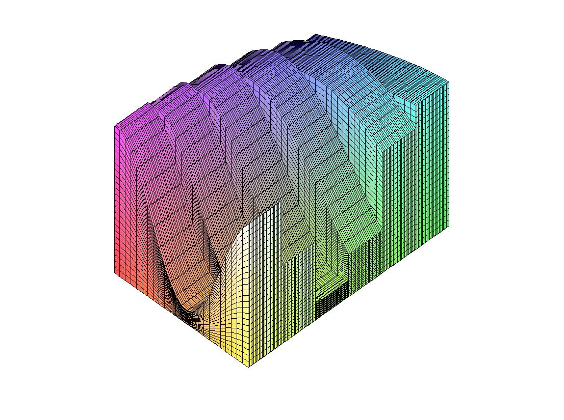
Going back to the double sum, we can rewrite it to emphasize a particular order in which we want to add the terms: $$\sum_{i=0}^{n-1}\left(\sum_{j=0}^{m-1}f(x_j,y_i)\Delta x\right)\Delta y.$$ In the sum in parentheses, only the value of $x_j$ is changing; $y_i$ is temporarily constant. As $m$ goes to infinity, this sum has the right form to turn into an integral: $$\lim_{m\to\infty}\sum_{j=0}^{m-1}f(x_j,y_i)\Delta x = \int_a^b f(x,y_i)\,dx.$$ So after we take the limit as $m$ goes to infinity, the sum is $$ \sum_{i=0}^{n-1}\left(\int_a^b f(x,y_i)\,dx\right)\Delta y. $$ Of course, for different values of $y_i$ this integral has different values; in other words, it is really a function applied to $y_i$: $$G(y)=\int_a^b f(x,y)\,dx.$$ If we substitute back into the sum we get $$\sum_{i=0}^{n-1} G(y_i)\Delta y.$$ This sum has a nice interpretation. The value $G(y_i)$ is the area of a cross section of the region under the surface $f(x,y)$, namely, when $y=y_i$. The quantity $G(y_i)\Delta y$ can be interpreted as the volume of a solid with face area $G(y_i)$ and thickness $\Delta y$. Think of the surface $f(x,y)$ as the top of a loaf of sliced bread. Each slice has a cross-sectional area and a thickness; $G(y_i)\Delta y$ corresponds to the volume of a single slice of bread. Adding these up approximates the total volume of the loaf. (This is very similar to the technique we used to compute volumes in section 8.3, except that there we need the cross-sections to be in some way "the same''.) Figure 17.1.3 shows this "sliced loaf'' approximation using the same surface as shown in figure 17.1.2. Nicely enough, this sum looks just like the sort of sum that turns into an integral, namely, $$\eqalign{ \lim_{n\to\infty}\sum_{i=0}^{n-1} G(y_i)\Delta y&=\int_c^d G(y)\,dy\cr &=\int_c^d \int_a^b f(x,y)\,dx\,dy.\cr }$$ Let's be clear about what this means: we first will compute the inner integral, temporarily treating $y$ as a constant. We will do this by finding an anti-derivative with respect to $x$, then substituting $x=a$ and $x=b$ and subtracting, as usual. The result will be an expression with no $x$ variable but some occurrences of $y$. Then the outer integral will be an ordinary one-variable problem, with $y$ as the variable.
Example 17.1.1 Figure 17.1.2 shows the function $\sin(xy)+6/5$ on $[0.5,3.5]\times[0.5,2.5]$. The volume under this surface is $$\int_{0.5}^{2.5}\int_{0.5}^{3.5} \sin(xy)+{6\over5}\,dx\,dy.$$ The inner integral is $$\int_{0.5}^{3.5} \sin(xy)+{6\over5}\,dx= \left.{-\cos(xy)\over y}+{6x\over5}\right|_{0.5}^{3.5}= {-\cos(3.5y)\over y}+{\cos(0.5y)\over y}+{18\over5}.$$ Unfortunately, this gives a function for which we can't find a simple anti-derivative. To complete the problem we could use Sage or similar software to approximate the integral. Doing this gives a volume of approximately $8.84$, so the average height is approximately $8.84/6\approx 1.47$. $\square$
Because addition and multiplication are commutative and associative, we can rewrite the original double sum: $$ \sum_{i=0}^{n-1}\sum_{j=0}^{m-1}f(x_j,y_i)\Delta x\Delta y=\sum_{j=0}^{m-1}\sum_{i=0}^{n-1}f(x_j,y_i)\Delta y\Delta x. $$ Now if we repeat the development above, the inner sum turns into an integral: $$\lim_{n\to\infty}\sum_{i=0}^{n-1}f(x_j,y_i)\Delta y = \int_c^d f(x_j,y)\,dy,$$ and then the outer sum turns into an integral: $$\lim_{m\to\infty}\sum_{j=0}^{m-1}\left(\int_c^d f(x_j,y)\,dy \right)\Delta x = \int_a^b\int_c^d f(x,y)\,dy\,dx.$$ In other words, we can compute the integrals in either order, first with respect to $x$ then $y$, or vice versa. Thinking of the loaf of bread, this corresponds to slicing the loaf in a direction perpendicular to the first.
We haven't really proved that the value of a double integral is equal to the value of the corresponding two single integrals in either order of integration, but provided the function is reasonably nice, this is true; the result is called Fubini's Theorem.
Example 17.1.2 We compute $\ds\dint{R} 1+(x-1)^2+4y^2\,dA$, where $R=[0,3]\times[0,2]$, in two ways.
First, $$\eqalign{ \int_0^3\int_0^2 1+(x-1)^2+4y^2\,dy\,dx&= \int_0^3\left. y+(x-1)^2y+{4\over 3}y^3\right|_0^2\,dx\cr &=\int_0^3 2+2(x-1)^2+{32\over 3}\,dx\cr &=\left. 2x + {2\over 3}(x-1)^3+{32\over 3}x\right|_0^3\cr &=6+{2\over 3}\cdot 8 + {32\over 3}\cdot3-(0-1\cdot{2\over3}+0)\cr &=44.\cr }$$ In the other order: $$\eqalign{ \int_0^2\int_0^3 1+(x-1)^2+4y^2\,dx\,dy&= \int_0^2\left. x+{(x-1)^3\over3}+4y^2x\right|_0^3\,dy\cr &=\int_0^2 3+{8\over3}+12y^2+{1\over3}\,dy\cr &=\left. 3y+{8\over3}y+4y^3+{1\over3}y\right|_0^2\cr &=6+{16\over3}+32+{2\over3}\cr &=44.\cr }$$ $\square$
In this example there is no particular reason to favor one direction over the other; in some cases, one direction might be much easier than the other, so it's usually worth considering the two different possibilities.
Frequently we will be interested in a region that is not simply a rectangle. Let's compute the volume under the surface $x+2y^2$ above the region described by $0\le x\le1$ and $0\le y\le x^2$, shown in figure 17.1.4.
In principle there is nothing more difficult about this problem. If we imagine the three-dimensional region under the surface and above the parabolic region as an oddly shaped loaf of bread, we can still slice it up, approximate the volume of each slice, and add these volumes up. For example, if we slice perpendicular to the $x$ axis at $x_i$, the thickness of a slice will be $\Delta x$ and the area of the slice will be $$ \int_0^{x_i^2} x_i+2y^2\,dy. $$ When we add these up and take the limit as $\Delta x$ goes to 0, we get the double integral $$\eqalign{ \int_0^1 \int_0^{x^2} x+2y^2\,dy\,dx&= \int_0^1 \left.xy+{2\over3}y^3\right|_0^{x^2}\,dx\cr &=\int_0^1 x^3+{2\over3}x^6\,dx\cr &=\left. {x^4\over4}+{2\over21}x^7\right|_0^1\cr &={1\over4}+{2\over21}={29\over84}.\cr }$$ We could just as well slice the solid perpendicular to the $y$ axis, in which case we get $$\eqalign{ \int_0^1 \int_{\sqrt y}^1 x+2y^2\,dx\,dy&= \int_0^1 \left.{x^2\over2}+2y^2x\right|_{\sqrt y}^1 \,dy\cr &=\int_0^1 {1\over2}+2y^2-{y\over2}-2y^2\sqrt y\,dy\cr &=\left. {y\over2}+{2\over3}y^3-{y^2\over4}-{4\over7}y^{7/2}\right|_0^1\cr &={1\over2}+{2\over3}-{1\over4}-{4\over7}={29\over84}.\cr }$$ What is the average height of the surface over this region? As before, it is the volume divided by the area of the base, but now we need to use integration to compute the area of the base, since it is not a simple rectangle. The area is $$\int_0^1 x^2\,dx={1\over3},$$ so the average height is $29/28$.
Example 17.1.3 Find the volume under the surface $\ds z=\sqrt{1-x^2}$ and above the triangle formed by $y=x$, $x=1$, and the $x$-axis.
Let's consider the two possible ways to set this up: $$\int_0^1 \int_0^x \sqrt{1-x^2}\,dy\,dx \qquad\hbox{or}\qquad \int_0^1 \int_y^1 \sqrt{1-x^2}\,dx\,dy. $$ Which appears easier? In the first, the inner integral is easy, because we need an anti-derivative with respect to $y$, and the entire integrand $\ds\sqrt{1-x^2}$ is constant with respect to $y$. Of course, the outer integral may be more difficult. In the second, the inner integral is mildly unpleasant—a trig substitution. So let's try the first one, since the first step is easy, and see where that leaves us. $$\int_0^1 \int_0^x \sqrt{1-x^2}\,dy\,dx= \int_0^1 \left. y\sqrt{1-x^2}\right|_0^x\,dx= \int_0^1 x\sqrt{1-x^2}\,dx. $$ This is quite easy, since the substitution $u=1-x^2$ works: $$\int x\sqrt{1-x^2}\,dx=-{1\over 2}\int \sqrt u\,du =-{1\over3}u^{3/2}=-{1\over3}(1-x^2)^{3/2}. $$ Then $$\int_0^1 x\sqrt{1-x^2}\,dx=\left. -{1\over3}(1-x^2)^{3/2}\right|_0^1 ={1\over3}. $$ This is a good example of how the order of integration can affect the complexity of the problem. In this case it is possible to do the other order, but it is a bit messier. In some cases one order may lead to a very difficult or impossible integral; it's usually worth considering both possibilities before going very far. $\square$
Exercises 17.1
Sage can compute many antiderivatives and so do many definite integrals. Since answers are given for the exercises, this in itself is not particularly useful. However, if you get the wrong answer to an exercise, it may not be obvious whether you have set up the integral incorrectly, or you have set it up correctly but then done the computation incorrectly. In such cases, you can try to use Sage to evaluate your integral to see if the answer matches the answer in the book.
Ex 17.1.1 Compute $\ds \int_{0}^{2}\int_{0}^{4} 1+x \,dy\,dx$. (answer)
Ex 17.1.2 Compute $\ds \int_{-1}^{1}\int_{0}^{2} x+y\,dy\,dx$. (answer)
Ex 17.1.3 Compute $\ds \int_{1}^{2}\int_{0}^{y} xy \,dx\,dy$. (answer)
Ex 17.1.4 Compute $\ds \int_{0}^{1}\int_{y^2/2}^{\sqrt y} \,dx\,dy$. (answer)
Ex 17.1.5 Compute $\ds \int_{1}^{2}\int_{1}^{x} {x^2\over y^2}\,dy\,dx$. (answer)
Ex 17.1.6 Compute $\ds \int_{0}^{1}\int_{0}^{x^2} {y\over e^x}\,dy\,dx$. (answer)
Ex 17.1.7 Compute $\ds \int_{0}^{\sqrt{\pi/2}}\int_{0}^{x^2} x\cos y\,dy\,dx$. (answer)
Ex 17.1.8 Compute $\ds \int_{0}^{\pi/2}\int_{0}^{\cos\theta}r^2 (\cos\theta-r) \,dr\,d\theta$. (answer)
Ex 17.1.9 Compute: $\ds \int_0^1\int_{\sqrt{y}}^1 \sqrt{x^3+1}\,dx\,dy$. (answer)
Ex 17.1.10 Compute: $\ds \int_0^1\int_{y^2}^1 y\sin(x^2)\,dx\,dy$. (answer)
Ex 17.1.11 Compute: $\ds \int_0^1 \int_{x^2}^1 x\sqrt{1+y^2}\,dy\,dx$ (answer)
Ex 17.1.12 Compute: $\ds \int_0^1 \int_0^y {2\over\sqrt{1-x^2}}\,dx\,dy$ (answer)
Ex 17.1.13 Compute: $\ds \int_0^1 \int_{3y}^3 e^{x^2}\,dx\,dy$ (answer)
Ex 17.1.14 Compute $\ds \int_{-1}^1\int_0^{1-x^2} x^2-\sqrt{y}\,dy\,dx$. (answer)
Ex 17.1.15 Compute $\ds \int_{0}^{\sqrt2/2}\int_{-\sqrt{1-2x^2}}^{\sqrt{1-2x^2}} x\,dy\,dx$. (answer)
Ex 17.1.16 Evaluate $\ds\dint{} x^2\,dA$ over the region in the first quadrant bounded by the hyperbola $xy=16$ and the lines $y=x$, $y=0$, and $x=8$. (answer)
Ex 17.1.17 Find the volume below $z=1-y$ above the region $-1\le x\le 1$, $0\le y\le 1-x^2$. (answer)
Ex 17.1.18 Find the volume bounded by $z=x^2+y^2$ and $z=4$. (answer)
Ex 17.1.19 Find the volume in the first octant bounded by $y^2=4-x$ and $y=2z$. (answer)
Ex 17.1.20 Find the volume in the first octant bounded by $y^2=4x$, $2x+y=4$, $z=y$, and $y=0$. (answer)
Ex 17.1.21 Find the volume in the first octant bounded by $x+y+z=9$, $2x+3y=18$, and $x+3y=9$. (answer)
Ex 17.1.22 Find the volume in the first octant bounded by $x^2+y^2=a^2$ and $z=x+y$. (answer)
Ex 17.1.23 Find the volume bounded by $4x^2+y^2=4z$ and $z=2$. (answer)
Ex 17.1.24 Find the volume bounded by $z=x^2+y^2$ and $z=y$. (answer)
Ex 17.1.25 Find the volume under the surface $z=xy$ above the triangle with vertices $(1,1,0)$, $(4,1,0)$, $(1,2,0)$. (answer)
Ex 17.1.26 Find the volume enclosed by $y=x^2$, $y=4$, $z=x^2$, $z=0$. (answer)
Ex 17.1.27 A swimming pool is circular with a 40 meter diameter. The depth is constant along east-west lines and increases linearly from 2 meters at the south end to 7 meters at the north end. Find the volume of the pool. (answer)
Ex 17.1.28 Find the average value of $f(x,y)=e^y\sqrt{x+e^y}$ on the rectangle with vertices $(0,0)$, $(4,0$), $(4,1)$ and $(0,1)$. (answer)
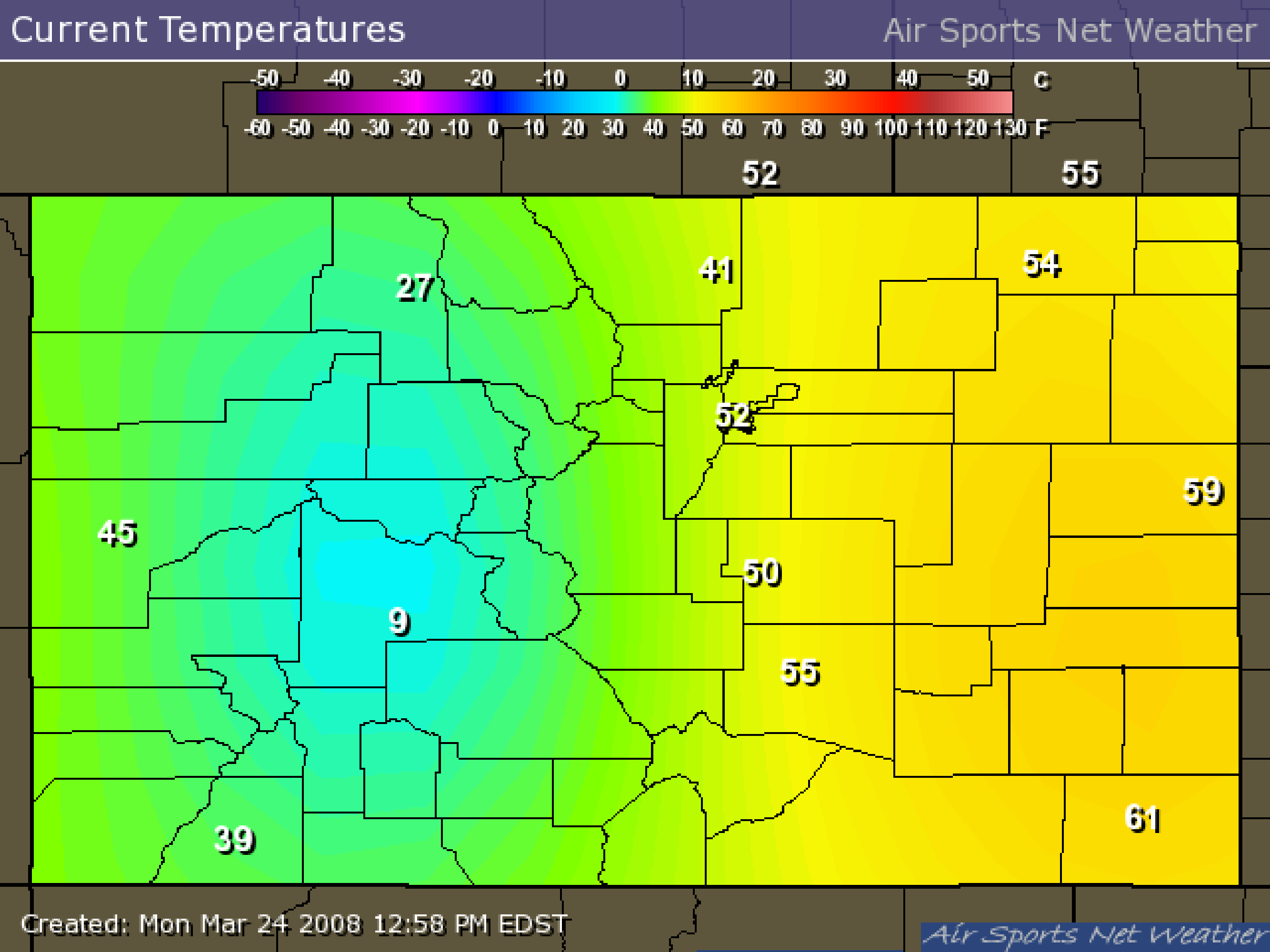
Ex 17.1.29 Figure 17.1.5 shows a temperature map of Colorado. Use the data to estimate the average temperature in the state using 4, 16 and 25 subdivisions. Give both an upper and lower estimate. Why do we like Colorado for this problem? What other state(s) might we like?
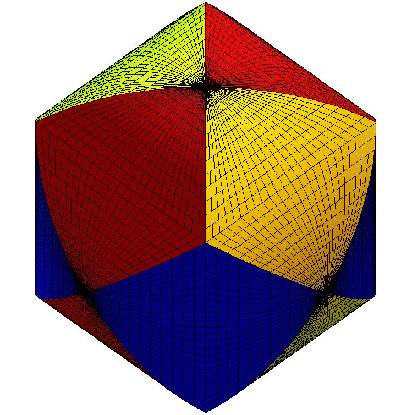
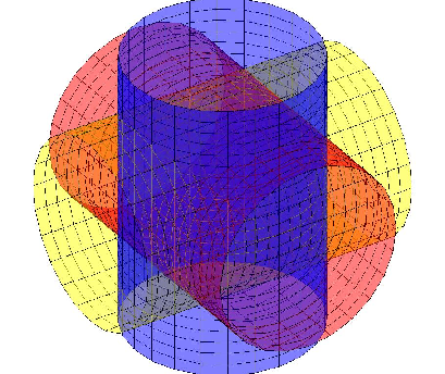
Ex 17.1.30 Three cylinders of radius 1 intersect at right angles at the origin, as shown in figure 17.1.6. Find the volume contained inside all three cylinders. (answer)
|
|
Ex 17.1.31 Prove that if $f(x,y)$ is integrable and if $\ds g(x,y)=\int_a^x \int_b^y f(s,t) \; dt \; ds$ then $g_{xy}=g_{yx}=f(x,y)$.
Ex 17.1.32 Reverse the order of integration on each of the following integrals
a. $\ds\int_0^9\int_0^{\sqrt{9-y}} f(x,y)\;dx\;dy$
b. $\ds\int_1^2\int_0^{\ln x} f(x,y)\;dy\;dx $
c. $\ds\int_0^1\int_{\arcsin y}^{\pi/2} f(x,y)\;dx\;dy$
d. $\ds\int_0^1\int_{4x}^{4} f(x,y)\;dy\;dx$
e. $\ds\int_0^3\int_{0}^{\sqrt{9-y^2}} f(x,y)\;dx\;dy$
(answer)
Ex 17.1.33 What are the parallels between Fubini's Theorem and Clairaut's Theorem (16.6.2)?